How to Profit from Increased Volatility in the Market

The first four inputs are known variables. To get number five, we plug those four inputs into the Black-Scholes model. This would give us “theoretical” implied volatility, which helps us decide if an option is cheap or expensive.

But given that options trade regularly, there is already an “actual” implied volatility assigned to each option, based on its price, which is constantly updating in real-time. Therefore, our mission — should we choose to accept it — is to determine whether an option’s current price looks cheap, or expensive based on its volatility level.

High or Low? Depends?

IV has a major impact on trading. To simplify this idea, let’s look at an example:

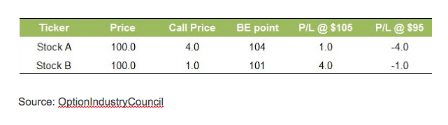
Stock A is priced at $100 and has high implied volatility. Let’s say that the call strike 100 costs $4.

Stock B is also priced at $100 but has low implied volatility. Let’s say that the call strike 100 costs $1.

When comparing the two trades, we can see that the break-even point of stock A is $104 and for stock B is $101. This means that we have a 1% increase to show profit in stock B, but 4% in stock A. Furthermore, if we assume a similar increase, let’s say 5% in each stock (by expiration) — we can see that there’s a $1 profit in stock A, but a $4 profit in stock B.

The following Table summarizes the two scenarios:

About the Author:

More...